Confidence Intervals and Coverage
Confidence Interval (CI)
- CI is an interval.
- An interval which is exepected to contain the parameter being estimated (eg: population mean.)
- Typical confidence levels are 95% and 99%.
- The confidence level of a confidence interval is called Nominal coverage (probability.)
- CI with 95% confidence: random interval which contains the parameter to be estimated 95% of the time.
- Two ways to mention a confidence level of 95%:
- Confidence interval with \(\gamma = 0.95\); 95% confidence
- Confidence interval with \(\alpha = 0.05\); 95% confidence: \(1-\alpha = 0.95\)
-
Mathematical representation
\[P(u(X)<\theta <v(X))=\gamma\]- \(\theta\) is the parameter to be estimated (eg: population mean or median).
- \(X\) is a random variable from a probability distribution with parameter \(\theta\)
- \(u(X)\) and \(v(X)\) are random variables containing parameter \(\theta\) with probability \(\gamma\)
- Confidence level \(\gamma\) < 1 (but close to 1). eg: 0.95
-
Mathematical representation in case of normal distribution:
\[\text{CI} = \bar{x} \pm z^* \left(\frac{\sigma}{\sqrt{n}}\right)\]Where:
- \(\bar{x}\) is the sample mean.
- \(z^*\) is the critical value corresponding to the desired confidence level
- \(\sigma\) is the population standard deviation.
- \(n\) is the sample size.
- The quantity \(\displaystyle {\sigma }_{\bar {x}}={\frac {\sigma }{\sqrt {n}}}\) is also called the standard error of the mean.
- The 95% confidence level will correspond to the 97.5th percentile of the distribution. Reason: the probability of \(\theta\) lying outside the 95% confidence level is 5%. So, 2.5% probability on both sides (if symmetric). So the range becomes 2.5% to (95+2.5)%.
- We can calculate the critical value \(z^*\) as follows:
- If the sample size is small (< 30) or we do not know the std dev, then we use the t-statistic (Student’s t-distribution.) The t-distribution is wider and has heavier tails than the normal distribution, reflecting the increased uncertainty in small samples. Thus, it accounts for the extra variability.
- If the sample size is large enough to make CLT valid, we use normal distribution (Z-distribution) –> z-score. Eg: a z-score of 1.96 for a 95% confidence level.
- As the sample size increases, both methods converge.
- It is better to use the t-statistic.
- Ref:
CI Width
- The narrower the width, the higher the confidence.
- Factors that impact the width of CI are sample size, variance/standard deviation, and confidence level.
- Sample size high –> narrow CI
- High variance/standard dev –> wider CI
- Higher confidence level –> wider CI (more data will lie under a higher confidence level)
Coverage
- Coverage (probability): the probability that a confidence interval will include the true value (eg: population mean.)
- The proportion of CIs (at a particular confidence level) that contain the true value (eg: population mean.)
- 95% CI coverage: For example, if you calculate a 95% confidence interval for a population mean, you are saying that if you were to take many samples and calculate a confidence interval from each one, approximately 95% of those intervals would contain the true population mean.
- Probability matching: if coverage probability is the same as nominal coverage probability.

- Nominal coverage = 50%
- Coverage = 10/20 = 50% (blue CIs contain the true mean)
- Probability matching since coverage is the same as nominal coverage.
- Image ref
- Ref:
Implementation and Explorations
Now, we will go through the above concepts in code.
Common imports
1
2
3
import numpy as np
import scipy.stats as st
import matplotlib.pyplot as plt
Compute CI
We implement the t-distribution and standard normal distribution to calculate the critical value.
1
2
3
4
5
6
7
8
9
10
11
12
13
14
15
16
17
18
19
20
21
22
23
24
25
26
27
28
29
30
31
32
def confidence_interval_t(sample, confidence=0.95):
    """
    Calculate the confidence interval for the mean of a sample using the t-distribution.

    This function is appropriate when the population standard deviation is unknown and
    the sample size is small (n < 30), although it works for any sample size.

    Parameters:
    sample (numpy.ndarray): The sample data as a NumPy array.
    confidence (float): The desired confidence level (default
    is 0.95 for a 95% confidence interval).

    Returns:
    tuple: Lower and upper bounds of the confidence interval.
    """
    # Ensure the sample is a NumPy array
    sample = np.array(sample)

    sample_mean = sample.mean()
    # Use Bessel's correction (ddof=1) for sample standard deviation
    sample_std = sample.std(ddof=1)
    sample_size = len(sample)
    standard_error = sample_std / np.sqrt(sample_size)

    # Determine the critical value for the specified confidence level
    critical_value = st.t.ppf((1 + confidence) / 2, df=sample_size - 1)
    margin_of_error = critical_value * standard_error

    lower_bound = sample_mean - margin_of_error
    upper_bound = sample_mean + margin_of_error

    return lower_bound, upper_bound
We use stats.t.ppf to get the critical value using the t-distribution. We can replace that with stats.norm.ppf for the z-score.
Confidence interval using standard normal distribution
1
2
3
4
5
6
7
8
9
10
11
12
13
14
15
16
17
18
19
20
21
22
23
24
25
26
27
28
29
30
31
32
33
34
def confidence_interval_norm(sample, confidence=0.95):
    """
    Calculate the confidence interval for the mean of a sample using the normal
    distribution (Z-distribution).

    This function is appropriate when the population standard deviation is
    known, or when the sample size is large (n >= 30), allowing the
    Central Limit Theorem to approximate the sample mean's distribution as normal.

    Parameters:
    sample (numpy.ndarray): The sample data as a NumPy array.
    confidence (float): The desired confidence level (default
    is 0.95 for a 95% confidence interval).

    Returns:
    tuple: Lower and upper bounds of the confidence interval.
    """
    # Ensure the sample is a NumPy array
    sample = np.array(sample)

    sample_mean = sample.mean()
    # Use Bessel's correction (ddof=1) for sample standard deviation
    sample_std = sample.std(ddof=1)
    sample_size = len(sample)
    standard_error = sample_std / np.sqrt(sample_size)

    # Determine the critical value for the specified confidence level
    critical_value = st.norm.ppf((1 + confidence) / 2)
    margin_of_error = critical_value * standard_error

    lower_bound = sample_mean - margin_of_error
    upper_bound = sample_mean + margin_of_error

    return lower_bound, upper_bound
Let’s compare the results with scipy implementations.
1
2
3
4
5
6
7
8
9
10
11
12
13
14
15
16
17
18
19
20
21
sample = np.random.random_sample(10)

print("defined functions:")
print("tstat:\t", confidence_interval_t(sample))
print("norm:\t", confidence_interval_norm(sample))

print("scipy functions:")
interval = st.t.interval(
    confidence=0.95, df=len(sample) - 1, loc=np.mean(sample), scale=st.sem(sample)
)
print("tstat:\t", interval)

interval = st.norm.interval(confidence=0.95, loc=np.mean(sample), scale=st.sem(sample))
print("norm:\t", interval)

# defined functions:
# tstat: (0.2756144976802315, 0.7458592632198344)
# norm:	 (0.3070236240157737, 0.7144501368842922)
# scipy functions:
# tstat: (0.2756144976802315, 0.7458592632198344)
# norm:	 (0.3070236240157737, 0.7144501368842922)
It is the same. In the following sections, we will use the scipy functions.
CI T-distribution vs. CI Z Distribution
We will verify if the confidence interval converges as the sample size increases in both methods. We will try both on the samples generated using the following sampling methods:
- Uniform
- Standard normal
- Poisson
1
2
3
4
5
6
7
8
9
10
11
12
13
14
15
16
17
18
19
20
21
22
23
24
25
26
27
28
29
30
31
32
33
34
35
sample_sizes = []
sample_means = []

t_interval_95_l = []
t_interval_95_r = []

norm_interval_95_l = []
norm_interval_95_r = []

for sample_size in range(10, 100, 5):
    sample = np.random.random_sample(sample_size)
    t_interval_95 = st.t.interval(
        confidence=0.95, df=len(sample) - 1, loc=np.mean(sample), scale=st.sem(sample)
    )
    norm_interval_95 = st.norm.interval(
        confidence=0.95, loc=np.mean(sample), scale=st.sem(sample)
    )
    sample_sizes.append(sample_size)
    sample_means.append(np.mean(sample))
    t_interval_95_l.append(t_interval_95[0])
    t_interval_95_r.append(t_interval_95[1])
    norm_interval_95_l.append(norm_interval_95[0])
    norm_interval_95_r.append(norm_interval_95[1])
    # print(sample_size, t_interval_95, norm_interval_95)

fig, ax = plt.subplots(figsize=(10, 5))
_ = ax.fill_between(
    sample_sizes, t_interval_95_l, t_interval_95_r, color="b", alpha=0.4
)
_ = ax.fill_between(
    sample_sizes, norm_interval_95_l, norm_interval_95_r, color="r", alpha=0.4
)
_ = ax.set_xlabel("Sample size")
_ = ax.set_ylabel("CI upper and lower bounds")
_ = ax.set_title("Uniform Distribution")
Replace np.random.random_sample with np.random.standard_normal and np.random.poisson to get standard normal and the Poisson random samples.
Here are the results:
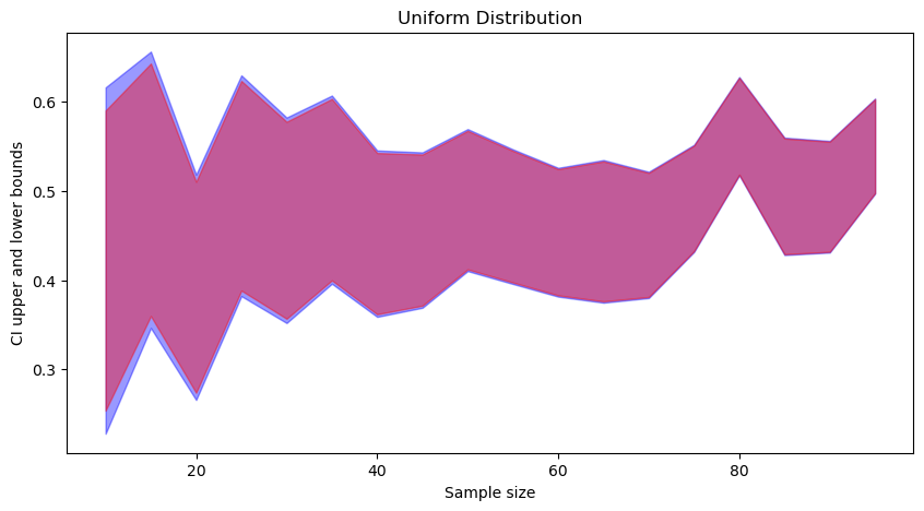
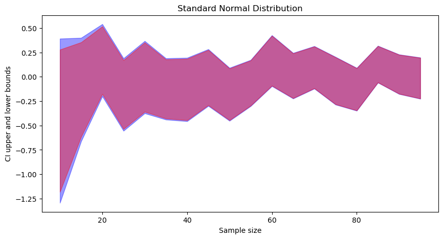
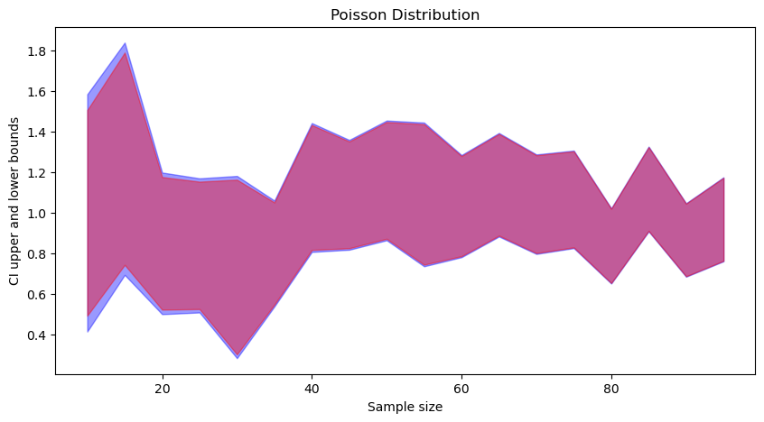
In each figure (click to zoom), the blue part corresponds to t-distribution-based CI, and the red part is to standard normal based CI. We can observe that:
- t-distribution based CIs are wider than standard normal based CI.
- As the sample size increases, both converge.
CI Width Simulations
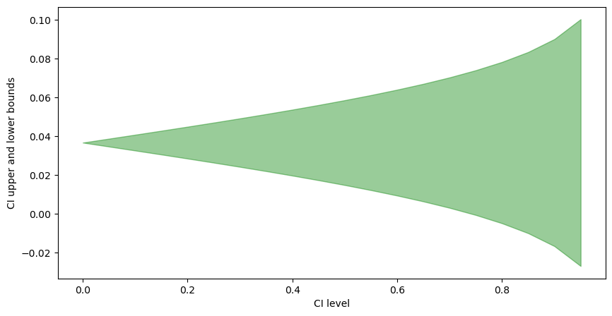
Let’s visualise how the CI width changes with different factors: confidence level, sample size, and standard deviation or variance.
Confidence Level - \(\gamma\)
The width of CI increases as the CI level increases. Intuition: as the confidence level increases, we widen the range to get the upper and lower limits of the confidence interval.
Code
1
2
3
4
5
6
7
8
9
10
11
12
13
14
15
16
17
18
19
20
sample = np.random.standard_normal(size=1000)
sample_mean = np.mean(sample)
sample_sem = st.sem(sample)

cis = []
t_interval_l = []
t_interval_r = []
for ci in range(0, 100, 5):
    ci = ci * 0.01
    t_interval = st.t.interval(
        confidence=ci, df=len(sample) - 1, loc=sample_mean, scale=sample_sem
    )
    cis.append(ci)
    t_interval_l.append(t_interval[0])
    t_interval_r.append(t_interval[1])

fig, ax = plt.subplots(figsize=(10, 5))
_ = ax.fill_between(cis, t_interval_l, t_interval_r, color="g", alpha=0.4)
_ = ax.set_xlabel("CI level")
_ = ax.set_ylabel("CI upper and lower bounds")
Sample Size
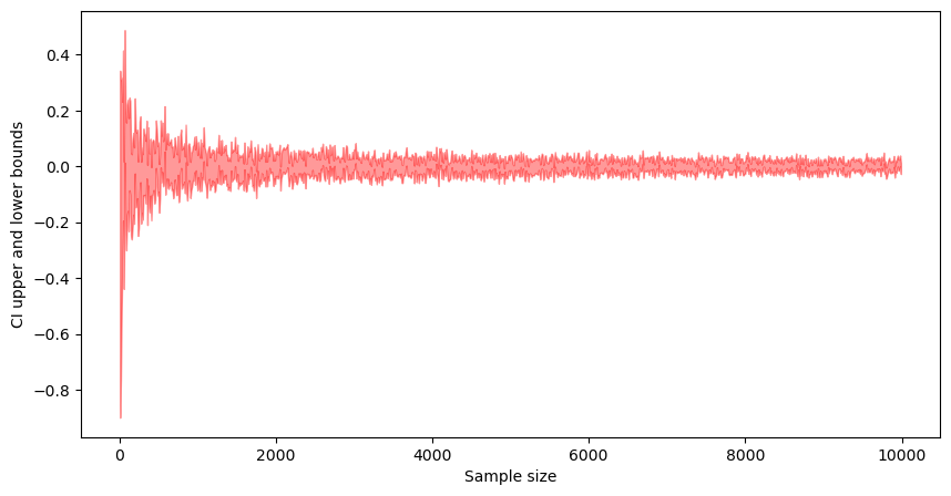
The width of CI reduces with as the sample size increases. Intuition: as sample size increases, we get more confident in our normal distribution parameter estimation, and thus, the confidence interval width reduces.
Code
1
2
3
4
5
6
7
8
9
10
11
12
13
14
15
16
17
18
19
20
21
22
23
24
25
sample_sizes = []
sample_means = []

t_interval_95_l = []
t_interval_95_r = []

norm_interval_95_l = []
norm_interval_95_r = []

for sample_size in range(10, 10000, 10):
    sample = np.random.standard_normal(size=sample_size)
    t_interval_95 = st.t.interval(
        confidence=0.95, df=len(sample) - 1, loc=np.mean(sample), scale=st.sem(sample)
    )
    sample_sizes.append(sample_size)
    sample_means.append(np.mean(sample))
    t_interval_95_l.append(t_interval_95[0])
    t_interval_95_r.append(t_interval_95[1])

fig, ax = plt.subplots(figsize=(10, 5))
_ = ax.fill_between(
    sample_sizes, t_interval_95_l, t_interval_95_r, color="r", alpha=0.4
)
_ = ax.set_xlabel("Sample size")
_ = ax.set_ylabel("CI upper and lower bounds")
Standard Deviation (Variance)
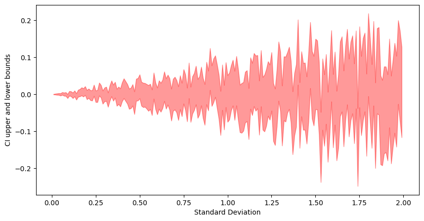
As with confidence level as the variance increases, we have more dispersion in the data. That leads to a wider CI width.
Code
1
2
3
4
5
6
7
8
9
10
11
12
13
14
15
16
17
18
19
20
21
22
23
stds = []
sample_means = []

t_interval_95_l = []
t_interval_95_r = []

norm_interval_95_l = []
norm_interval_95_r = []

for std in range(0, 200, 1):
    std = std * 0.01
    sample = np.random.normal(loc=0, scale=std, size=1000)
    t_interval_95 = st.t.interval(
        confidence=0.95, df=len(sample) - 1, loc=np.mean(sample), scale=st.sem(sample)
    )
    stds.append(std)
    t_interval_95_l.append(t_interval_95[0])
    t_interval_95_r.append(t_interval_95[1])

fig, ax = plt.subplots(figsize=(10, 5))
_ = ax.fill_between(stds, t_interval_95_l, t_interval_95_r, color="r", alpha=0.4)
_ = ax.set_xlabel("Standard Deviation")
_ = ax.set_ylabel("CI upper and lower bounds")
Probability Matching
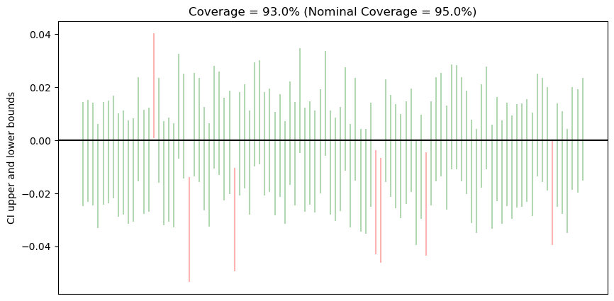
Coverage probability will not always be the same as nominal coverage probability. When it matches, we get probability matching. In the below figure, out of 100 confidence intervals, 7 CIs do not contain the true mean (black.) Thus, we get a coverage of 93%, which is not the same as 95%, hence no probability matching.
Code
1
2
3
4
5
6
7
8
9
10
11
12
13
14
15
16
17
18
19
20
21
22
23
24
25
26
27
28
29
30
31
32
33
34
35
population = np.random.standard_normal(size=100000)

ci_ids = []
t_interval_l = []
t_interval_r = []
ci_contains_true_value = []

ci_level = 0.95
for i in range(100):
    sample = np.random.choice(population, size=10000, replace=False)
    t_interval = st.t.interval(
        confidence=ci_level,
        df=len(sample) - 1,
        loc=np.mean(sample),
        scale=st.sem(sample),
    )
    ci_ids.append(i + 1)
    t_interval_l.append(t_interval[0])
    t_interval_r.append(t_interval[1])

    if t_interval[0] <= 0 <= t_interval[1]:
        ci_contains_true_value.append(1)
    else:
        ci_contains_true_value.append(0)

cols = ["g" if i == 1 else "red" for i in ci_contains_true_value]
fig, ax = plt.subplots(figsize=(10, 5))
_ = ax.vlines(ci_ids, t_interval_l, t_interval_r, color=cols, alpha=0.3)
_ = ax.axhline(0, color="black")
_ = ax.set_ylabel("CI upper and lower bounds")
_ = ax.set_xticks([])
_ = ax.set_title(
    f"Coverage = {sum(ci_contains_true_value) * 100 / len(ci_contains_true_value)}%"
    f" (Nominal Coverage = {ci_level*100}%)"
)
Conclusion
A Confidence Interval is an interval over a sample that is expected to contain the distribution parameter that we are trying to estimate (eg: mean.) That means that all CIs will not contain the mean. The sample and population mean could have the following properties:
- It does not contain the mean
- It contains the mean somewhere in the middle
- It contains the mean but as an outlier
Since the confidence interval is built from this sample using normal distribution the confidence interval may not contain the mean in the 1st or the 3rd scenario. That is why we take the confidence level as 95% or more to handle the 3rd scenario (demonstrated in the simulation section).
Since narrow-width confidence intervals are better (and more reliable), we should try to
- take higher confidence levels (95% or more);
- have a bigger sample size; and
- have less variance in the data.